Numerical Simulation: Definition, Discretization, DoFs


Deepak S Choudhary
Numerical simulation turns a real engineering system into a mathematical model, discretizes it into finite degrees of freedom, and then solves for state variables to predict outputs you can design against.
Why This Matters
Numerical simulation is not a “nice-to-have” plot generator. It is a decision tool that helps you choose geometry, materials, and operating limits before you pay for hardware iterations.
The value shows up when physical prototypes are expensive or slow, and one automotive virtual development report notes drivable prototypes can cost on the order of $500,000 to $1,000,000 per unit, with many prototypes in a program. (reposiTUm)
Numerical Simulation Definition And Governing Model
Numerical simulation is used to find approximate solutions to engineering problems by first formulating system behavior as a mathematical model, typically PDEs under specified boundary conditions.
The important part is what the model actually contains. This framework frames an engineering problem using three sets of variables:
I= system inputsS= system characteristics or parametersO= system outputs
The system behavior is represented implicitly as:
This is a compact way of saying: given inputs and characteristics, the outputs must satisfy the governing physics and constraints.
Plain-English recap: if I and S are vague or wrong, O will be confidently wrong, because the solver can only enforce what you actually told it.
Problem Domain Vs Solution Domain
Most pages online stop at “simulation solves the model.” This goes one level deeper, which is what engineers trust: it separates the problem domain from the solution domain using degrees of freedom (DoFs).
In the problem domain, the real system lives in a continuous space. In principle, that means infinite DoFs because points in a continuum are uncountable. In the solution domain, you build a discretized model with a finite number of DoFs, and you solve explicitly for those state variables.
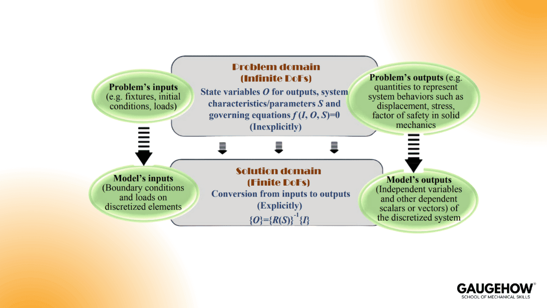
A simple “engineer’s translation” of this Fig is:
Problem inputs (fixtures, initial conditions, loads) become model inputs (boundary conditions, applied loads on discretized entities).
Problem outputs (stress, displacement, safety factor, temperature) become computed outputs from solved state variables.
The solver is the conversion engine that maps boundary conditions to state variables and then to outputs.
Decision-Aid Visual To Include
Place a single flow diagram right here (as your hero figure), based directly on Fig. 3.7:
Inputs I + Characteristics S → Governing Equation (1) → Discretization → Finite DoFs → Solve State Variables → Outputs O
That visual is not decorative. It prevents “black-box” use because it forces the reader to name what is input, what is state, and what is output.
Input–State–Output Traceability Ledger
Competitors rarely give engineers a traceability artifact. Add this compact table as a reusable “credibility ledger” for any simulation:
Ledger Row | What To Write | Example (Structure) | Why It Matters |
Inputs | Loads, fixtures, initial conditions |
| Defines what the solver must satisfy |
Characteristics | Material, geometry parameters |
| Controls stiffness and field response |
Outputs | Decision outputs |
| Must map to a pass/fail requirement |
DoF Count | nodes × variables |
| Predicts cost and sensitivity to mesh |
Plain-English recap: if you cannot fill this ledger in 60 seconds, you are not ready to trust the contour plot.
What Discretization Actually Changes
In practice, the simulation model differs from the real problem in four specific ways. That list is the practical heart of numerical simulation, because it explains why simulations can be both powerful and fragile.
First, discretization replaces a continuous domain with a discrete representation, where node behaviors represent the field. Second, the discretized model has a limited number of DoFs, and each DoF corresponds to a state variable to be solved. Third, the model must be solvable so that state variables are found explicitly under the specified boundary conditions and loads. Fourth, parameters are split so that boundary conditions and loads are defined on discretized entities while other dependent quantities are treated as state variables or outputs.
Plain-English recap: numerical simulation is not “solving the real thing.” It is solving a finite, discretized proxy whose credibility depends on how you choose the discretization and constraints.
Numerical Methods Used In Practice
Numerical simulation sits under computational methods, used when the system is too complex or uncertain for graphic, experimental, or closed-form analysis. It then highlights three common numerical method families engineers run into:
Finite Element Analysis (FEA)
Finite Difference Method (FDM)
Boundary Element Method (BEM)
The operational difference is where the unknowns live. FEA discretizes the entire domain using elements and nodes. BEM discretizes only the boundary, which can reduce modeling effort when boundary behavior dominates. It also separates methods by how they treat derivatives. FEA forms equations through element-level integration, while FDM approximates derivatives at grid points using finite differences.
Plain-English recap: choose the method based on where the physics “lives,” not based on what your team happens to know already.
Worked Micro-Example With Numbers: From PDE To DoFs
This example is intentionally small so an engineer can reproduce it quickly and see the full I → S → O chain.
Problem Statement
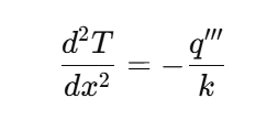
A 1D slab of length L = 0.10 m has uniform volumetric heat generation q'' = 1.0×10^6 W/m^3 and constant thermal conductivity k = 200 W/(m·K). Boundary temperatures are fixed: T(0)=0 °C, T(L)=0 °C.
The governing equation is:
Discretization Into DoFs
Use 5 nodes (including boundaries), so spacing is:
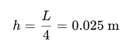
Unknowns are the internal node temperatures T_1, T_2, T_3. That is 3 DoFs because the boundary nodes are prescribed.
Using the standard central difference:
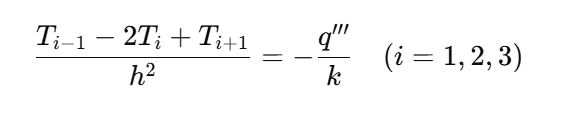
Rearrange:
With q'''/k = 5000 K/m^2 and h^2 = 0.000625 m^2, the right side is 3.125 K.
Solve And Interpret Outputs
With T_0 = 0 °C and T_4 = 0 °CThe solved internal temperatures are:
T_1 = 4.6875 °CT_2 = 6.25 °CT_3 = 4.6875 °C
So the peak output is T_max ≈ 6.25 °C at mid-span.
Plain-English recap: you started with a PDE and boundary conditions, then turned it into 3 solvable DoFs, and those DoFs produced a decision-grade output (T_max) with explicit units.
Simulation Workflow Engineers Trust
A practical simulation process almost always follows three phases: preprocessing, solving, and postprocessing. Siemens describes this as a typical CAE flow where you define geometry and physical properties plus loads or constraints, solve using an appropriate physics formulation, then review results in postprocessing. (Siemens Digital Industries Software)
From an operational standpoint, the common failure mode is not “the solver is wrong.” It is that preprocessing silently encoded the wrong problem, so the solver faithfully solved the wrong thing. Postprocessing can then make the wrong answer look convincing if you never trace outputs back to I, S, and DoFs.
A simple trust workflow is:
State the ledger: write
I,S, and targetObefore meshing.Choose discretization to control DoFs and gradients, not just to “make it run.”
Confirm outputs are derived from state variables that are actually constrained by your boundary conditions.
Plain-English recap: the fastest way to improve simulation credibility is to make the model definition explicit, then refuse to proceed when the ledger is incomplete.
Key Technical Points
Numerical simulation becomes credible when you can name
I,S, andOand tie them to the governing model (f(I, S, O )=0), because that prevents hidden assumptions from becoming “results.”
Discretization is the fundamental approximation step, so treat mesh and DoF choices as physics choices, not as geometry chores, because they determine what the solver can represent.
Finite DoFs mean you are solving for state variables on nodes or elements, so every added field variable multiplies computational cost and should be justified by a decision need.
Use FEA when interior field variation matters and you need a general-purpose domain method, but consider boundary-focused approaches like BEM only when boundary behavior drives theresponsee and the method assumptions actually hold.
Prefer a small reproducible check like the micro-example before trusting a full model, because it forces the full chain from PDE to DoFs to outputs with units and sanity bounds.
Engineer Takeaways & Action Checklist
Write the Input–State–Output ledger before you mesh, and do not proceed until each output maps to a pass/fail requirement, with units and a target tolerance documented.
Track DoFs explicitly for every run, and record the runtime and peak memory alongside DoFs, with the acceptance criterion that performance trends must be explainable by DoF changes and physics settings.
Verify boundary conditions are applied to the intended entities and directions, with the acceptance criterion that reaction forces or heat balance match expectations within an agreed residual limit for the model type. (Siemens Digital Industries Software)
Run one “known-shape” micro-check (like a 1D conduction case) before large 3D models, with the acceptance criterion that the solver reproduces the known peak value or trend within the chosen tolerance.
Choose the numerical method family based on where unknowns live, with the acceptance criterion that the discretization aligns with the physics domain and boundary dominance assumptions.
Keep a single page of model intent stating.
I,S,O, and the governing equation form, with the acceptance criterion that any reviewer can reproduce the model definition without opening the solver GUI.
FAQ
What Makes A Simulation “Numerical” Instead Of Analytical?
Analytical methods aim for closed-form expressions you can evaluate directly, which typically limits them to simpler geometries and boundary conditions. Numerical simulation replaces that with a discretized model that yields approximate solutions computed from finite DoFs.
Are PDEs Always Required For Numerical Simulation?
Most engineering simulation is PDE-driven because fields vary over space and time, and the solver only becomes well-posed once you apply boundary conditions. Lumped-parameter dynamics can also be simulated numerically, but the credibility discipline around inputs, state, and outputs still applies.
Why Do Boundary Conditions Matter So Much?
They define the constrained problem you are actually solving. Treat loads and boundary conditions as primary inputs that close the problem and determine the state variables, because any mistake here changes the physics you actually solve.
Conclusion
Numerical simulation is best understood as a controlled conversion: from a real engineering system with continuous behavior to a discretized, solvable model with finite DoFs. I, S, O Framing and the problem-domain vs solution-domain split are the practical anchors because they force traceability from boundary conditions and parameters to solved state variables and decision outputs.
When you treat discretization as the core approximation step, keep inputs explicit, and validate outputs against what the model can actually represent, numerical simulation becomes a repeatable engineering method rather than an attractive visualization. That is how you win time, reduce prototype churn, and make decisions earlier with less regret.
How To Implement
Step 1: Write the ledger (I, S, target O, DoFs estimate) and the governing equation form you are assuming.
Step 2: Discretize to match gradients and decision outputs, then solve the smallest reproducible check case before scaling up.
Step 3: Review results by tracing each output back to state variables and boundary conditions, then record DoFs, runtime, and acceptance checks for the run.
References
Siemens Digital Industries Software, “Computer-aided engineering (CAE)” (preprocessing, solving, postprocessing). (Siemens Digital Industries Software)
MIT OpenCourseWare, “Introduction to Numerical Simulation (6.336J)” course page. (MIT OpenCourseWare)
Wikipedia, “Finite difference method” (canonical definition of FDM as derivative approximation). (Wikipedia)
K. Selvam, Virtual Product Development: A method to reduce lead time… (prototype cost ranges and program prototype counts in an automotive context). (reposiTUm)
CAD-CAM-CAE Work Platform
Find or Post CAD, CAM and CAE freelance projects, full-time jobs and Internships.
GaugeHow is the platform built for core engineering work. Whether you need a freelancer for a CAD project, a full-time hire, or an engineering intern,post it here and get matched with the right person.
Our Courses
Complete Course Library
Access to 40+ courses covering various fields like Design, Simulation, Quality, Manufacturing, Robotics, and more.