Absorbing Boundary Conditions For Seismic Analysis In Abaqus

If your soil model edges reflect energy, your interior histories can look clean but wrong. This guide shows absorbing boundary conditions for seismic analysis in Abaqus by comparing absorber types, then giving a truly zero-guess viscous implementation for Standard and Explicit, plus a reflection ratio and an energy sign check so results stand up in review.

You can run a dynamic soil model and still be misled by it. The reason is simple. When you truncate an “infinite” ground into a finite mesh, outgoing waves hit artificial edges and come back as reflections. Those reflections can add late peaks, shift the phase, and create a tail that looks like real damping or real amplification.

Most pages ranking for this topic fall into two extremes. One extreme is paper-first content that explains frameworks but does not remove implementation ambiguity. The other extreme is quick tips that say “add dampers” but never tell you how to size them per node or prove they reduced reflections.

This page is written the way a reviewer reads. First, you choose an absorber approach quickly. Then you implement the most practical baseline, the Lysmer–Kuhlemeyer viscous idea, with both keywords and CAE path,s so nobody is blocked by workflow. Finally, ly you verify it with a reflection ratio, and one extra energy sign sanity check, so you can defend the boundary, not just hope it worked.

Absorber Options 

Most real projects do not fail because the absorber theory is unknown. They fail because the absorber is underspecified, misdirected, or never verified.

If you want one stable baseline that is quick to audit, the viscous option is still the practical starting point in many models because it targets impedance matching directly.

Viscous Absorber Fundamentals You Can Trust

The core idea is impedance matching. For a traveling wave, traction is proportional to particle velocity through the medium impedance.

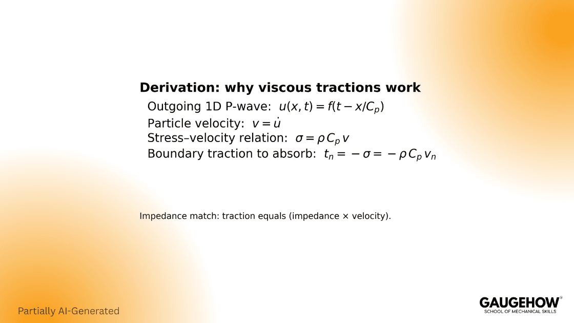
If you apply a traction that is equal and opposite to that traveling-wave traction, you remove energy instead of reflecting it.

This is the intuition behind the classic Lysmer–Kuhlemeyer boundary:

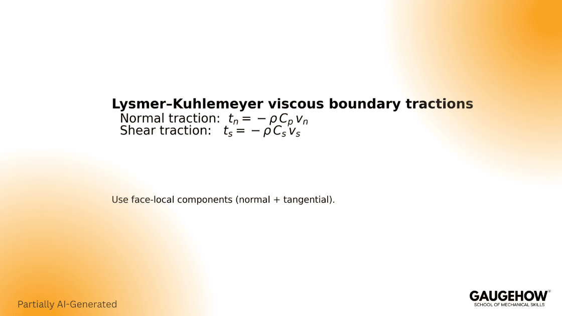
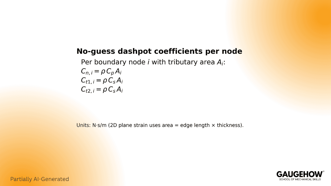
In its common engineering form for a boundary face, you size dashpots with:

Where (Ai) is the node tributary boundary area (or edge length times thickness in 2D plane strain). This “per node” mapping is what prevents the two most common failure modes: overdamping corners and underdamping mid-edge nodes.

One limitation you should state plainly for technical trust: viscous absorbers are most exact for body-wave content and are not perfect for all angles or strongly surface-wave-dominated cases.

How We Think Differently

A boundary condition is not “done” when it runs without errors. It is done when it produces the same interior decision after you change mesh density once, and when its energy behavior is consistent with physics.

Absorbing boundary conditions for seismic analysis in Abaqus

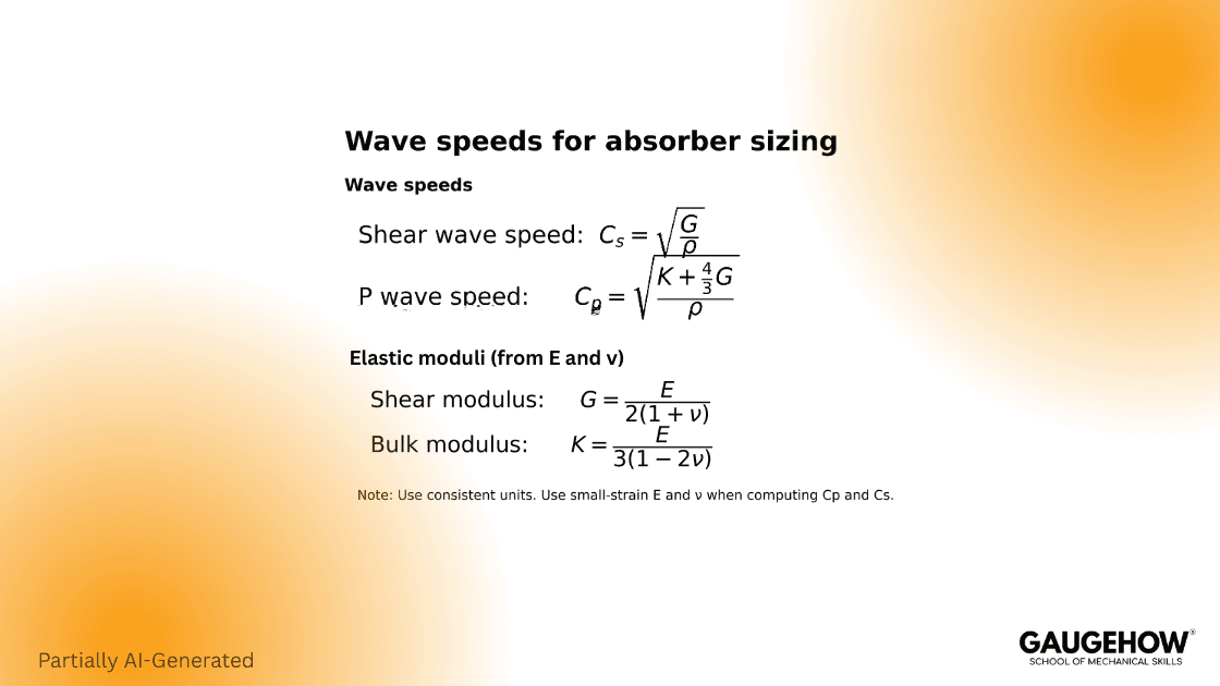
Step 1: Lock the Inputs That Control Impedance

Use small-strain stiffness for wave speeds. Then lock these four inputs before you touch Abaqus keywords:

Step 2: Compute Coefficients Per Boundary Node

For each boundary node:

If you only do a single “average” coefficient per edge, you create avoidable direction and corner errors. Your own draft already points to that node-by-node mapping, which is the correct framing.

Step 3: Implement With Keywords (No Guessing)

Abaqus/Standard: DASHPOT1(S) to ground (fixed DOF, with orientation)

Dashpot element availability matters. In Standard, DASHPOT1(S) is the “node to ground” style, and it supports directional definition through DOF and orientation.

Orientation (Local Coordinate System)

** -------------------------------------------------
** Local orientation for X-min boundary damping
** e1 = outward normal (global X)
** e2 = tangential direction 1 (global Y)
** e3 = tangential direction 2 (global Z)
** -------------------------------------------------
*ORIENTATION, NAME=ORI_XMIN, SYSTEM=RECTANGULAR
1., 0., 0., 0., 1., 0.

Normal Damping (Local Direction 1)

*ELEMENT, TYPE=DASHPOT1, ELSET=DP_XMIN_N

900001, 1001

*DASHPOT, ELSET=DP_XMIN_N, ORIENTATION=ORI_XMIN

1

2.40E+06

Tangential Damping – Direction 1 (Local Direction 2)

*ELEMENT, TYPE=DASHPOT1, ELSET=DP_XMIN_T1

900002, 1001

*DASHPOT, ELSET=DP_XMIN_T1, ORIENTATION=ORI_XMIN

2

1.20E+06

Tangential Damping – Direction 2 (Local Direction 3)

*ELEMENT, TYPE=DASHPOT1, ELSET=DP_XMIN_T2

900003, 1001

*DASHPOT, ELSET=DP_XMIN_T2, ORIENTATION=ORI_XMIN

3

1.20E+06

Where the coefficients land: in the *DASHPOT data, the coefficient is the numeric value under the DOF line for the element set.

Abaqus/Explicit: DASHPOTA (axial dashpot) between two nodes

This is a real reviewer gap in your earlier draft: it says Explicit can use “DASHPOT1 to ground,” which is not the clean, version-stable choice because DASHPOT1(S) is Standard-only and Explicit uses DASHPOTA for the axial dashpot pattern.

Dummy node (explicitly grounded)

*NODE
600001, -1.0, 0., 0. ** dummy node along outward normal

*BOUNDARY
600001, 1, 3, 0.0 ** FIXED: makes dashpot act to ground

Axial dashpot element

*ELEMENT, TYPE=DASHPOTA, ELSET=DP_XMIN_N_AX

910001, 500001, 600001

Dashpot definition

*DASHPOT, ELSET=DP_XMIN_N_AX

2.40E+06

For DASHPOTA linear behavior, the *DASHPOT block uses a blank first line and the coefficient on the next line.

Step 4: Implement In Abaqus/CAE 

Even if you prefer keywords, including this path wins because it removes workflow friction for readers.

CAE click path:
Property module or Interaction module → Special → Springs/Dashpots → Create (then select dashpot form and assign coefficient).

• Standard: choose “to ground” style (maps cleanly to DASHPOT1(S)).

• Explicit: choose an axial dashpot between two nodes (maps cleanly to DASHPOTA).

Step 5: Request The Outputs You Need For Verification

A dashpot is a relative-velocity force mechanism, so you must request variables that let you compute power and confirm dissipation.

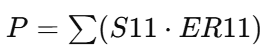
From the dashpot element library, S11 (dashpot force) is available, and ER11 (relative velocity) is available for Standard.

Reflection Ratio R and Energy Sign Sanity Check

Check 1: Reflection Ratio R (Keep your current structure, just tighten wording)

Use one sensor near the interior (incident) and one sensor closer to the boundary (reflected). Fix the time windows once using travel time logic, then do OFF vs ON with identical windows.

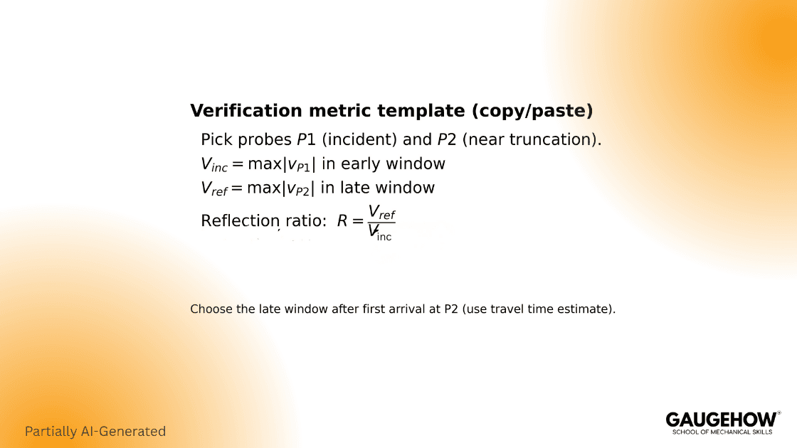
A practical baseline pass line many teams use for initial absorber validation is R less than or equal to 0.10. It is not universal, but it is repeatable and reviewable.

Check 2: Energy Sign Sanity Check (Dashpots must remove energy, not inject it)

Add this single line and your verification becomes harder to argue with:

Instantaneous boundary power should be non-positive

How to compute it in Abaqus:

• Standard: use dashpot element S11 and ER11, then:

  

  
  

• Explicit: compute relative velocity from nodal velocities of the two nodes of the axial dashpot (boundary node minus dummy node), then multiply by dashpot force.

If you see sustained positive power, the usual root causes are simple: the normal direction sign is flipped, the DOF mapping is wrong, or coefficients are assigned to the wrong face set.

Optional Fast Check That Engineers Like: Whole-Model Energy Trend

Request energy output and confirm the balance behaves sensibly. In Explicit workflows, the standard energy identifiers include ALLIE, ALLKE, ALLVD, ALLWK, ETOTAL, and the documented balance form ties them together (for example, ETOTAL combinations built from these terms). (WashU Engineering Classes)

This is not about chasing perfect conservation. It is about catching the ugly mistake quickly: an absorber that injects energy.

Hybrid Free-Field Coupling

Sometimes, viscous absorption alone is not enough because side boundaries must also move realistically with the incoming wavefield. That is where free-field coupling appears in the literature, including Nielsen’s framework work around extending Abaqus for seismic boundary handling.

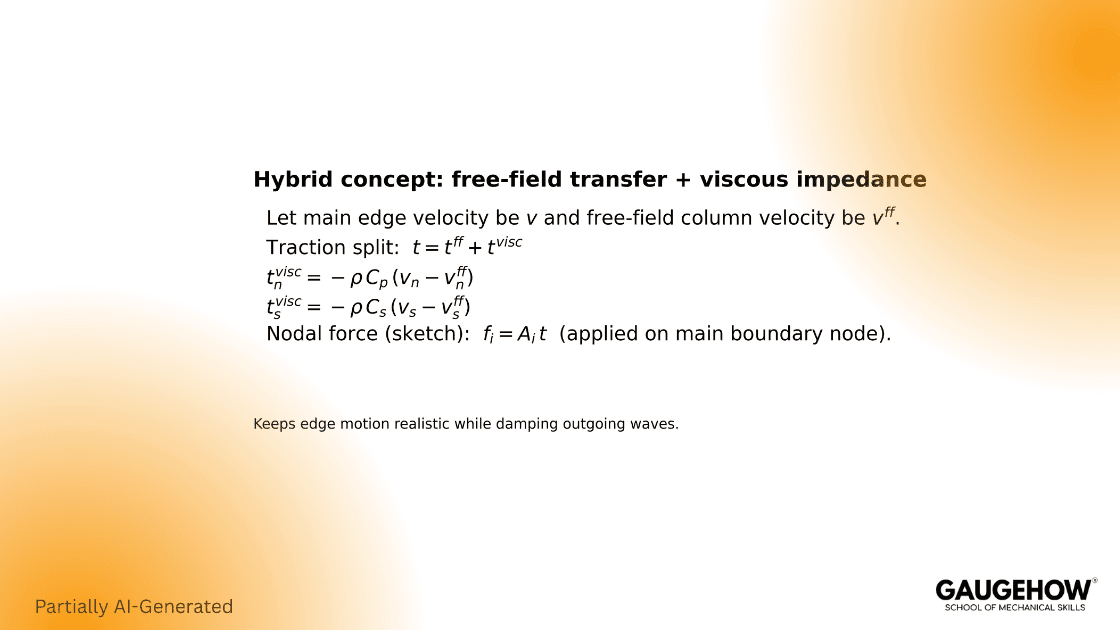
A buildable engineering statement of the hybrid idea is:

1. Pair each main boundary node with a node in a free-field column at the same elevation.

2. Split traction into a free-field transfer part plus a viscous impedance part acting on relative motion.

3. Implement the custom coupling through UEL so you return both the residual vector and a consistent tangent matrix, because that is what the UEL interface requires in Standard.

This is exactly where most write-ups lose people. They describe the concept but never state the contract your element must satisfy in Abaqus.

FAQ

How do I know if my boundary is reflecting too much?

Use one fixed reflection ratio definition with fixed windows, then compare OFF vs ON with the same probe locations. If the metric drops clearly and stays stable across a small mesh refinement, you can defend it.

Why do corners behave worse than straight edges?

Corners concentrate two error types: wrong tributary area mapping and direction ambiguity. That is why corner nodes are where you most often see overdamping or injected work.

What input mistake most often breaks viscous sizing?

Using softened or large-strain stiffness to compute wave speeds. Size from small-strain assumptions, then let the nonlinear model do its job after.

Can I use infinite elements instead of dashpots?

Sometimes yes, but you still must verify the interface behavior because the transition can reflect if the setup is inconsistent.

When should I consider free-field or hybrid coupling?

When realistic side motion matters as much as absorption, especially for layered profiles where boundary kinematics influence response.

References

• Abaqus Analysis User’s Manual, dashpot behavior and usage. WashU Engineering Classes+1
  
  

• Abaqus/Explicit dashpot element types and definition keywords. VT Software Docs
  
  

• Abaqus User Subroutines Reference Manual, UEL interface signature and required returns. WashU Engineering Classes+1
  
  

• Nielsen (2014), ICE Engineering and Computational Mechanics paper describing free-field tools and element extensions in Abaqus. Emerald+1
  
  

• Lysmer and Kuhlemeyer viscous boundary background and later efficiency correction discussion. ASCE Library+1

• Abaqus documentation mirrors: energy balance identifiers and relationships used for validation (ALLIE, ALLKE, ALLVD, ALLWK, ETOTAL). (WashU Engineering Classes)

Conclusion

You now have the theory, the implementation, and the proof checks. If your boundary absorbs energy, your interior results stay honest. Use these steps, then verify with the reflection ratio and energy sign. If you want faster industry-ready depth, explore our advanced FEA courses.