You will run one baseline case and then judge it. One KPI stays fixed, and the mesh stays defensible. Numerics remain conservative, and trends stay interpretable. A 30-minute acceptance gate keeps you from wasting compute.

After installing OpenFOAM, doubt is normal. Residuals can drop and still lie. That doubt helps, because you want evidence. Screenshots do not count as evidence.

This OpenFOAM tutorial is written like a review checklist. Run a case, and then judge it properly. That is the whole point.

One note before we start, to be honest with you. No tool guarantees perfect results. What stays under your control is clarity. Specificity also stays under your control, along with engineering judgment.

What OpenFOAM Really Is And Why Workflow Discipline Matters

OpenFOAM is an open-source CFD toolbox. It is built on finite volume methods. Cases are defined using text dictionaries, so changes remain traceable.

That structure supports reproducibility, which matters in real work. At the same time, a sloppy setup gets punished fast. Small mistakes often trigger big instability.

Most first-run failures are basic, not advanced. Weak mesh quality near gradients is common. Outlet backflow with no protection is also common. Aggressive numerics can look fast and then collapse suddenly. An undefined KPI creates noise chasing, too.

A professional workflow reduces uncertainty in stages. Debugging becomes faster because each change stays isolated. This matters because you want clear cause and effect.

The Case Structure You Must Understand First

Every OpenFOAM case uses three directories: 0, constant, and system. Each directory has one clear job. The 0 folder holds initial fields and boundary fields. The constant folder holds properties as well as mesh data. The system folder holds run controls and numerics.

Inside the systemThree files dominate outcomes in practice. Run control lives in controlDict. Discretization lives in fvSchemes. Solver settings and relaxation live in fvSolution.

From a review standpoint, treat these like a contract. If any part is vague, the solver will expose it. If any part is wrong, the result will drift.

Define Your Goal Before You Touch The Case

Before running anything, write two lines. Those two lines prevent most beginner mistakes.

First line: your physics assumptions. Decide whether it is incompressible or compressible. Decide whether steady or transient. Decide on the turbulence model and the property behavior too.

Second line: your KPI definition, with units. Pressure drop, mass flow, drag, lift, and peak temperature work well. Pick one KPI first, and add more later.

This framing prevents random tuning. It also makes the run review defensible. A solver log is not the result. A stable KPI trend is the result.

Pick Your First OpenFOAM Case: A Defensible Starter

A starter case should teach transferable habits. So choose a setup where errors show quickly. Choose a setup where the KPI is easy to extract from.

For your first OpenFOAM case, use a pressure drop duct or a bluff body. Both give measurable KPIs, so judgment becomes faster.

A duct teaches boundary discipline and wall modeling. A bluff body teaches separation behavior and force extraction. Both teach the same workflow logic, which is basically why they work.

Complex geometry can wait. Multiphase can wait, too, and rotating frames can wait. Early complexity hides fundamentals rather than teaching them.

OpenFOAM Workflow: Baseline Sequence

A baseline run is not your final answer. It is your first controlled experiment. Stability and interpretability come first.

Below is the OpenFOAM workflow you will reuse. Treat it as your run log, because it keeps your work repeatable.

Keep changes minimal in the baseline. One run should repeat cleanly. After that, change one variable per iteration cycle.

Table: CFD Workflow Step by Step: The Run Log Every Engineer Should Keep

That table is your backbone. Skipping steps removes your safety rails. Merging steps hides root causes.

CFD Workflow Step By Step: Do This In Order

A clean run uses two screens. Keep case files on one side. Keep solver logs on the other side. That habit makes debugging faster.

Step 1: Define the Physics Like a Design Review

Start with compressibility because it drives everything. If Mach is low, incompressible usually fits. Next, decide steady versus transient based on physics. When the flow is inherently unsteady, forcing steady can mislead.

Then choose turbulence modeling. For a first pass, a RANS baseline is practical. Debugging becomes easier, and the computational cost stays manageable.

After that, lock properties. Density and viscosity must match the temperature assumption. If the temperature is unknown, state a reference temperature and stick to it.

Finally, confirm the KPI and its extraction method. Internal flows usually use pressure drop. External flows often use drag or lift.

Step 2: Build a Baseline Mesh with Predictable Behavior

Early meshes should favor stability, not perfection. Predictable behavior matters more than fancy resolution.

Use blockMesh for the baseline with mild grading. Boundary layers do not need perfection yet. First, establish a stable workflow, and then improve resolution safely.

Keep refinement aligned with the KPI zone. That focus improves accuracy per cell.

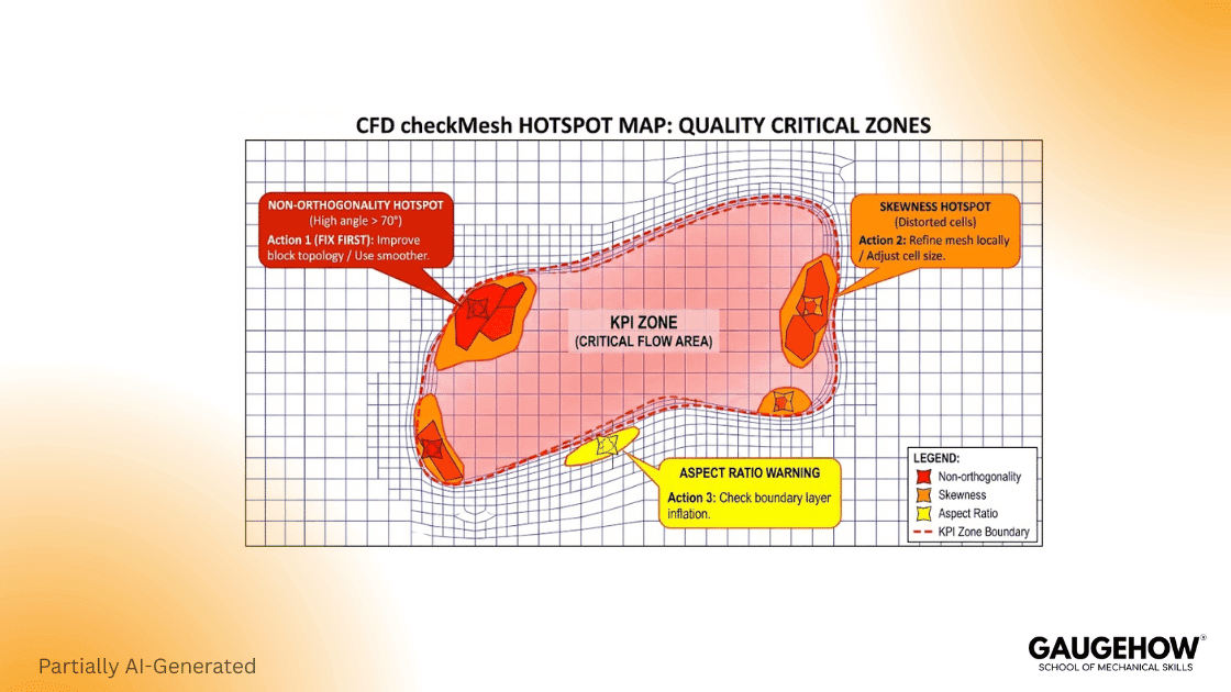
Step 3: Check Mesh Validity before Boundary Tuning

Mesh validation is a gate, not a suggestion. You want the worst cells and their locations.

Run checkMesh and locate the worst cells near the KPI. A mesh can pass checks and still be hostile near gradients.

If the worst cells sit in the KPI zone, fix them first. If they sit far away, proceed to the baseline. Either way, record the mesh summary.

Step 4: Set Boundaries as Physics, Not Defaults

Boundary setup defines physics and stability together. Begin with the physical driver. Decide if the inlet is velocity-driven, mass flow-driven, or pressure-driven.

Then anchor the domain with an outlet pressure reference. For external flow, use a far field that avoids reflections. For internal flow, keep the outlet stable and predictable.

Backflow deserves attention because it breaks many runs. If backflow can occur, outlet boundaries must handle return flow safely.

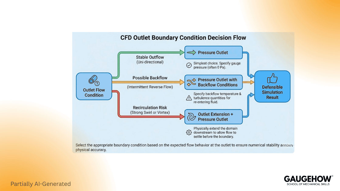
Design boundary conditions in OpenFOAM with backflow in mind. Ignoring backflow often looks like random divergence. It is not random; it is boundary behavior.

Step 5: Choose Numerics for Stability First

High-order schemes can backfire early. A conservative first run builds trust faster.

Set conservative discretization in fvSchemes. Keep the start boring and robust. Once stability is proven, accuracy can be improved systematically.

Choose robust linear solvers fvSolution with mild relaxation. High relaxation can appear fast, but it can fail suddenly. Mild relaxation stays slower, and it stays predictable.

When oscillations appear, check numerics and mesh first. Only after that should deeper physics be blamed.

Step 6: Pick the Solver that Matches the Problem

A steady incompressible baseline is usually the first step. Cost stays lower, and debugging stays clearer.

Use simpleFoam for steady incompressible baselines. When the KPI depends on transient history, use a transient solver and control the time step carefully.

Use pisoFoam when transient physics matters. A baseline is still the goal here. Perfection can wait.

Step 7: Run with Objective stop rules and a KPI trend

Runs should stop on evidence, not on feelings. Objective stop rules protect your time.

Add residual control logic for objective stops. Still, treat residuals as a health indicator only. The KPI trend is your acceptance signal.

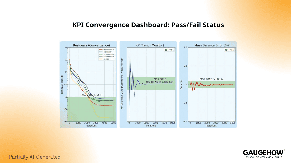
If residuals drop but KPI drifts, the run is not mature. If residuals stall but KPI stabilizes, the run may be mature. Both signals must agree.

Step 8: Post-process to answer one question at a time

Start with the KPI plot, and then add one supporting field view. Consistency matters more than visuals.

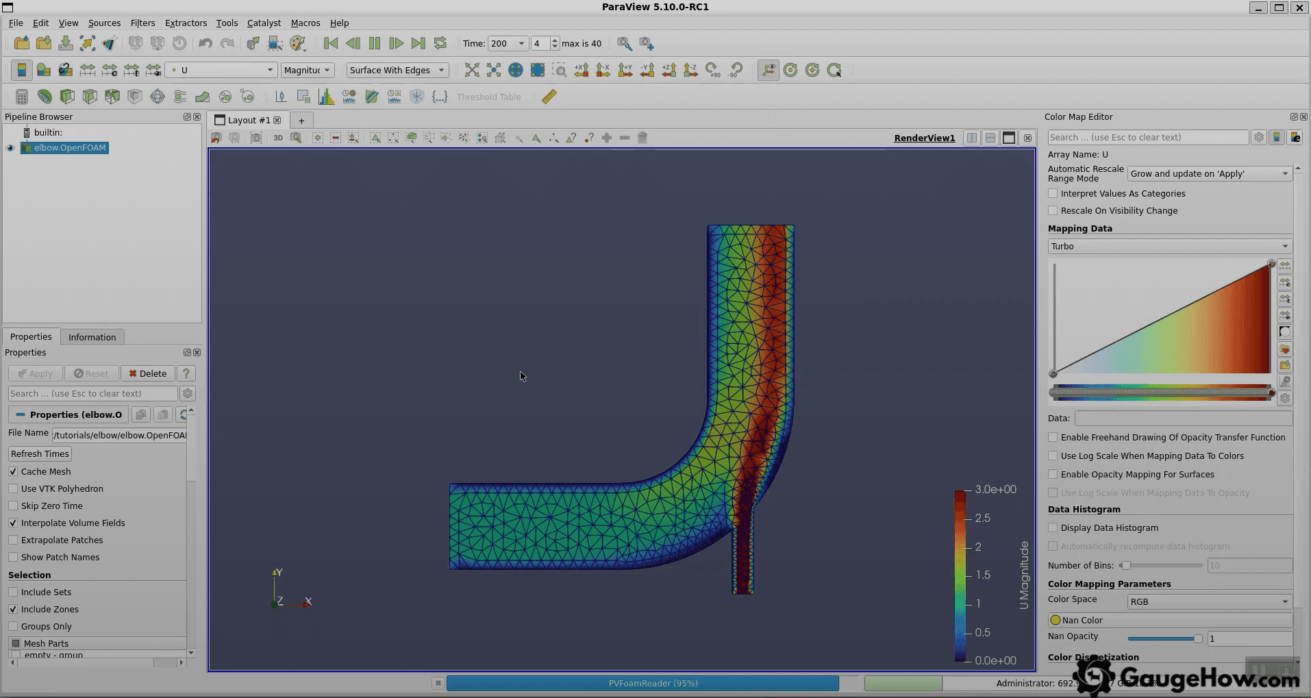
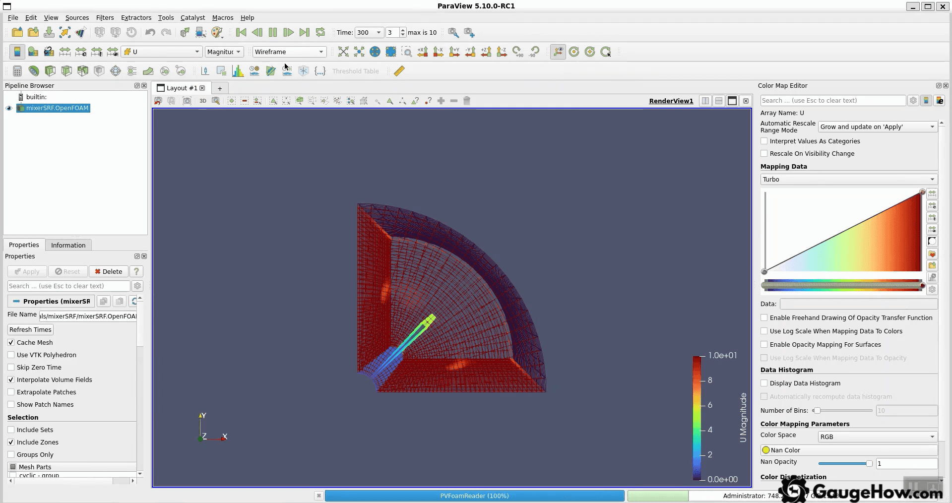
Use ParaView post-processing to automate KPI extraction. Repeatable plots keep comparisons clean. Clicking randomly makes workflows drift.

That is the CFD workflow step-by-step sequence: define, mesh, run, review, and verify.

The 30-minute Acceptance Gate That Saves Your Week

Many workflows stop at “it runs.” Real work needs a gate. A good gate is fast, repeatable, and decisive.

Run this gate after your first stable baseline. Do it before refinement. Do it before turbulence tweaks, too.

A Worked Mini Example You Can Actually Replicate

Concrete baselines teach faster than theory. A simple duct case is enough to build discipline.

Run a straight duct with a simple feature removed. Choose pressure drop as the KPI. Use incompressible and steady flow for the first pass. Set an inlet velocity that gives a clear Reynolds number. Keep properties constant and keep numerics conservative.

Now run three meshes, changing only mesh density. Keep physics and numerics unchanged. Extract the same pressure drop surfaces each time.

Table: Three Meshes with One KPI trend

That trend is what you want. The change shrinks with refinement. Sensitivity reduces, so confidence increases.

If the trend becomes chaotic, stop and diagnose. Mesh quality issues often cause it. Outlet behavior can cause it,t too, and inconsistent extraction can cause it as well.

What Actually Goes Wrong In Practice, And How You Respond

Real work fails in predictable ways. The trick is responding in the right order.

Common failures include these:

• Divergence after early progress, often from mesh hotspots.

• Backflow at the outlet is causing unstable return values.

• Residuals are dropping while KPI drifts slowly.

• Pressure reference mistakes shift absolute levels.

• Over-aggressive schemes cause oscillations and noise.

• Mis-scaled properties are pushing the wrong Reynolds regime.

• Bad patch naming, applying wrong boundaries.

• Wrong extraction surfacesare making the KPI meaningless.

Response logic should stay simple.

When the mesh report is severe, fix the mesh first. Tuning solvers on a broken mesh wastes time. Mesh repair is often the highest leverage step.

If checkMesh reports severe non-orthogonality, fix the mesh and rerun. Then recheck conservation and KPI stability.

When backflow appears, treat it as a boundary design issue. Solver blame is rarely correct here.

Many “solver issues” are actually poor boundary conditions in OpenFOAM. Fix outlet behavior, and then repeat the baseline.

If residuals drop but KPI drifts, run longer and review sampling. Stronger under relaxation may help, but change one lever at a time.

Slow and stable is fine early. Speed comes later, once sensitivity drivers are understood.

Solver Selection Clarity Without Confusion

A long solver catalog is not needed. One clean decision path is enough.

Use a steady incompressible baseline when the KPI is time-averaged. Use a transient solver only when the KPI depends on unsteady history. After choosing, lock it and stay consistent.

Table: Practical Solver Comparison

Both options still share the same anchors. The KPI is the decision metric. Conservation is the gate that blocks self-deception.

Best Practices That Keep Your Work Fast And Credible

Small habits create deliverable quality. These habits also prevent silent drift.

• Write a one-page case note with assumptions.

• Keep one KPI definition with clear units.

• Save KPI versus iteration or time plots.

• Log mesh quality summary for each run.

• Change one variable per iteration cycle.

• Archive the case folder before major changes.

Keep controlDict clean and predictable. Use residual control as a guardrail. Keep fvSchemes conservative early. Inspect fvSolution when oscillations persist.

Use blockMesh refinements focused on the KPI zone. Global refinement wastes cells fast.

Post-Processing That Stays Repeatable Across Runs

Repeatable extraction is part of the workflow, not an afterthought. Without it, comparisons become unreliable.

Use saved ParaView states when possible. Keep slice planes consistent across runs. Keep integration surfaces consistent, too.

Build scripts for ParaView post-processing if you can. Repeatability reduces human error, and it makes runs comparable.

Frequently asked questions

Do I need to master everything before my first run?

No. A stable baseline workflow matters more. One KPI and one acceptance gate are enough to start.

Why do residuals drop,p, but the result feels wrong?

Residuals are not correct. Check conservation and outlet behavior, along with KPI stability. The n verify sensitivity using a second mesh.

What should my first OpenFOAM case be?

Choose one KPI, one solver, and a simple mesh. Validate it with three meshes. Keep extraction surfaces consistent.

How do I stop wasting compute on a run?

Use objective stop rules and a KPI based gate. Do not let “it is still running” become the plan.

How should post-processing be handled for repeatability?

Automate extraction and reuse the same views. Lock the workflow early so comparisons remain valid.

This OpenFOAM tutorial keeps one principle central: start with one KPI and strict 0, constant, and system discipline. Everything else builds on that foundation.

Conclusion

A perfect first run is not required. A defensible baseline run is required.

This workflow forces clarity each time. One KPI stays fixed. Mesh validity is checked. Outlets are designed for backflow risk. Runs stop on objective rules. Sensitivity is verified with controlled changes.

Next step: choose one baseline and run the OpenFOAM workflow again. Keep the same run log discipline and build the habit.