Computational Fluid Dynamics: CFD Workflow and V&V Checks

If you encounter flow problems and need answers to defend, this guide is your map from first setup to trusted results. A CFD simulation works best when you treat it like controlled engineering work, because a clean-looking field can still be wrong if the domain, mesh, or modeling assumptions do not match the physics.

The workflow below is written the way I would brief a junior engineer at a workstation and also the way I would defend a decision in a design review. You will see what to decide, what to save, and where most projects quietly fail.

What are solving in CFD

At its core, Computational Fluid Dynamics solves conservation laws numerically. You enforce mass, momentum, and often energy across a discretized domain, and the solution only becomes physical when the modeling choices and inputs match the real situation. That is why accuracy is rarely won in post-processing and is almost always won earlier, in setup.

Governing equations you should keep in your head

For most engineering flows, you solve Navier–Stokes in some form. Continuity enforces mass conservation. Momentum balances forces with acceleration and viscous stress. Energy matters when temperature shifts density or properties.

You rarely solve the pure form in production work. Instead, you apply assumptions and closures so the problem is solvable with the compute and time you have, and then you verify that those assumptions do not dominate the decision.

Discretization is where accuracy is earned.

Most industrial solvers use the finite volume method, so conservation is built in when schemes are consistent. The practical consequence is simple: your answer depends on mesh resolution, mesh quality, and numerics, and a stable run is not proof of accuracy because stability can be purchased with numerical diffusion.

CFD workflow

In Computational Fluid Dynamics, you get faster by being consistent, because speed comes from fewer reruns rather than faster clicking, and a CFD simulation usually fails in predictable places when the process is rushed. The workflow is the same whether you run a duct pressure drop or an external aerodynamics case. What changes is the level of evidence you gather before you publish numbers.

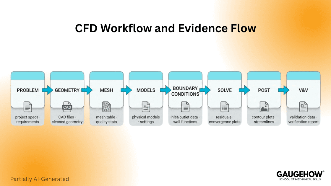
The process table you actually use

Practical guideline: if you cannot produce a saved artifact for a stage, pause, because auditability is what lets reviewers reproduce and trust your claim.

Stage gates that prevent wasted weeks

The same workflow becomes much easier to execute when you treat it as gates. Each gate has a pass criterion and a required artifact, so you do not discover fundamentals after a week of computing.

Problem definition: start with the decision

Before opening a solver, write one line that you could read aloud in a review, for example: “Predict pressure drop across this duct at 200 CFM within ±10%.” That sentence forces clarity on the operating point and what good enough means, and it prevents scope drift.

Separate the validation variable from the decision metric. You might validate ΔP, but decide based on temperature uniformity, and if you mix those up, you will end up defending the wrong thing later.

Geometry and domain: make boundaries stay out of the physics

A tight domain is one of the fastest ways to get believable but wrong results, because boundaries start acting like physical constraints. Domain sizing is not glamorous, but it is a first-order effect in external flows and a frequent hidden issue in internal flows.

Internal flows

For pipes, ducts, manifolds, and heat exchangers, include enough upstream length for profile development or prescribe a profile intentionally and document it. A short inlet with a uniform velocity can force an artificial development region that distorts losses.

External flows

For bluff-body cases, far-field placement influences drag and wake development, and cylinder studies show measurable sensitivity until boundaries are moved sufficiently far away. A practical starting point for 2D cylinder studies is upstream 10D, downstream 15D to 20D, and lateral at least 8D.

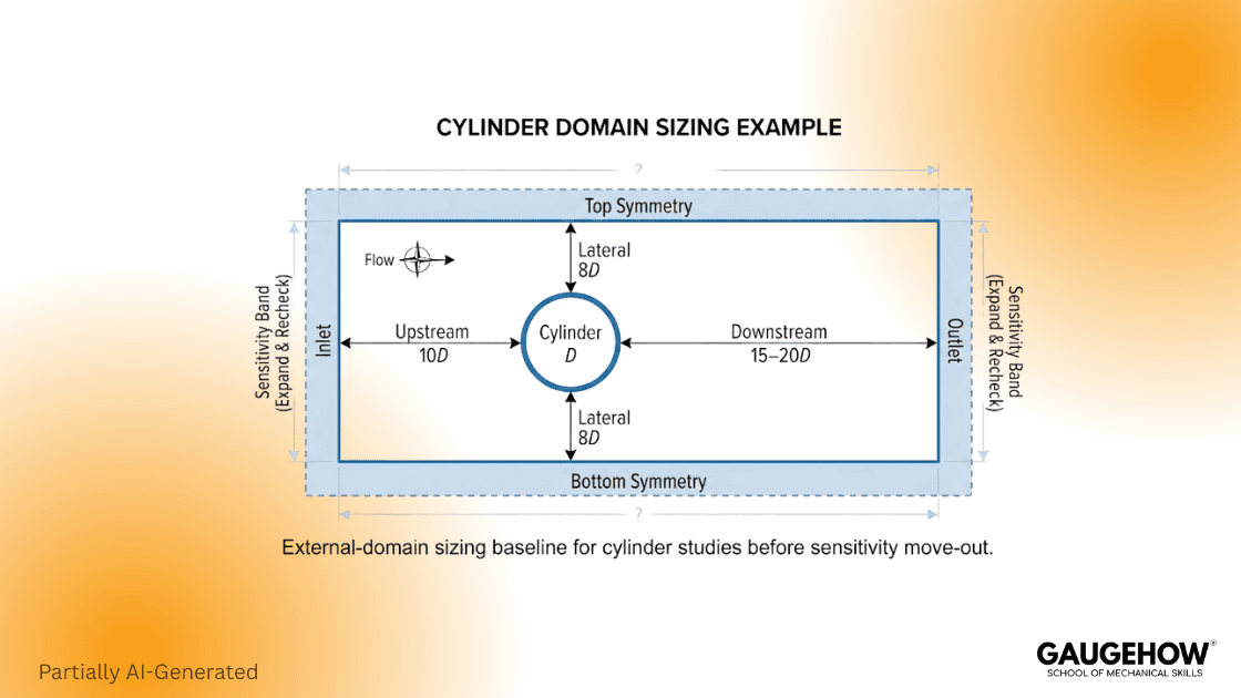
Practical guideline: if force coefficients change meaningfully when you move boundaries outward, your earlier domain was influencing the result, so expand and re-check.

Mesh: resolution is placement, not cell count

A large mesh can still be a poor mesh if it does not resolve the gradients that control the decision. Put resolution where physics lives, because uniform refinement wastes compute and still misses the important gradients.

What you are trying to resolve

You refine near walls for shear and heat transfer, around separation and reattachment, and in wakes and jets where mixing dominates. For compressible flow, shocks need focused refinement, and for multiphase flow, interfaces need resolution that matches the model assumptions.

Quality is not optional.

Skewness, non-orthogonality, and abrupt size transitions can create diffusion or instability. A stable run can be stabilized by numerical diffusion, so treat quality hotspots as first-class problems and fix them before you spend compute on sensitivity studies.

Near-wall planning

Near-wall resolution controls friction and heat transfer and also shifts separation behavior, so plan it rather than discovering it later. Use y+ as the design coordinate that links the first cell height and prism-layer growth to the wall treatment you selected.

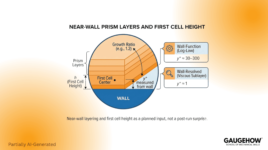
A practical starting point is to target values in the 30–300 range when using standard wall functions and target around 1 when you intend a wall-resolved approach, while avoiding accidental operation in the buffer region unless your solver’s near-wall treatment is designed for it.

Turbulence closures: match assumptions to the flow

Most engineering flows are turbulent, so you almost always rely on a closure model. The main failure mode here is not that a model is bad in general, but that the model assumptions are misaligned with the dominant physics and the near-wall strategy.

Use turbulence modeling language precisely in reports. Say which closure you used, what near-wall treatment you paired with it, and which outputs the decision depends on.

RANS, LES, DNS in practical terms

RANS is the production workhorse because it solves for the mean flow with modeled turbulent transport. LES resolves the larger unsteady structures and models smaller scales, so it is appropriate when unsteady dynamics drive the decision, and the budget allows. DNS resolves everything and is not practical for most engineering applications.

k–ε, k–ω, and SST without overselling

k–ε is often robust for many attached internal flows, but it can be optimistic in separation or strong adverse pressure gradients if the near-wall treatment is mismatched. k–ω is more sensitive near walls, and SST blends k–ω near the wall with k–ε away from the wall, which is why many teams prefer it as a default for separation risk, provided the mesh and wall treatment support it.

Boundary conditions: where most projects break

Boundary conditions define the problem you are solving, so be strict here. Document every boundary with type, magnitude, profile, turbulence inputs, temperature, roughness, and reference frames, because ambiguity is what creates non-reproducible results.

Boundary-condition table template

Practical guideline: treat mass imbalance above about 0.5% as a warning sign unless you can explain why it is acceptable for the decision, because conservation is the foundation, and it is the first thing reviewers use to challenge results.

Numerics and convergence: residuals are necessary, not sufficient

Residuals tell you the linear system is settling down. They do not guarantee that your engineering quantities are stable. Treat converged as a combination of iterative convergence and physical convergence.

Monitor what the decision depends on, such as ΔP, forces, outlet temperature, or flow split, and also monitor conservation (mass and energy, where relevant). This is the simplest protection against false convergence.

Common failure modes and fast checks

Most wrong answers come from a small set of causes, and that is why experienced teams develop a short reality check that they run before they trust contours. The point is not bureaucracy. The point is catching boundary-driven solutions, under-resolved gradients, and missing evidence while the fix is still cheap.

10-minute reality check before you publish 

• Confirm the objective, units, and operating point match the report and the solver inputs.

• Confirm the domain is not artificially tight, and that moving boundaries outward would not change the decision.

• Confirm the boundary conditions table is complete, including turbulence inputs and reference frames.

• Confirm that the near-wall plan is stated, including the wall treatment choice and the designed near-wall target.

• Confirm the engineering monitors used for the decision are flat, and conservation is acceptable.

• Confirm that at least one sensitivity check exists, typically a second mesh, and ideally three meshes for high-risk work.

A debug sequence that actually works

• Simplify physics until the case is stable and bounded, and then add complexity one element at a time.

• Use conservative, bounded discretization and modest relaxation, because stability beats speed during diagnosis.

• Reduce the time step for transients and pay attention to initialization, because bad initial fields create false instability.

• Fix mesh quality hotspots locally, because a few bad regions often dominate the whole run.

• Reintroduce higher-order schemes and tighter settings only after monitors behave sensibly.

How to defend results in a review

A reviewer is not looking for perfect certainty. They are looking for a clear chain of evidence that shows what you assumed, what you checked, and how sensitive the decision is to the things you could be wrong about.

What a reviewer expects on one page

• Objective and operating points, stated in plain language with units.

• Domain figure with key dimensions and boundary placement rationale.

• Mesh table with counts, quality metrics, and the near-wall strategy you designed.

• Model list, including the closure choice and any key constants you changed from defaults.

• Boundary conditions table with units, profiles, and turbulence inputs.

• Convergence evidence showing residuals and, more importantly, flat engineering monitors.

•  Verification and validation evidence, including mesh sensitivity and an uncertainty band, are required when the decision is at high risk.

Verification and validation: grid convergence, GCI, and evidence

This is where work becomes publishable. Verification and validation separate numerical correctness from physical correctness. Verification quantifies numerical error, while validation compares to data and frames how much trust you can place in absolute values.

A practical evidence set includes a mesh sensitivity study, a time-step study for transient runs, and clear convergence plots for the engineering outputs.

Mesh sensitivity

This section is where you convert “it looks converged” into a result you can defend, because you show how the answer moves with refinement and you report a bounded discretization estimate.

Worked Example 1: Pipe pressure drop with grid sensitivity and GCI

The purpose of this example is not the pipe. It involves a reporting workflow consisting of three meshes, a sensitivity table, and a transparent uncertainty band.

Problem setup

Fluid is water near 20°C. Pipe diameter D = 0.01 m and length L = 1.0 m. Reynolds number Re = 10,000. The target output is the pressure drop ΔP across 1 m.

At Re = 10,000, the average velocity is about 1.0 m/s. A smooth pipe correlation gives a Darcy friction factor near 0.032. That predicts ΔP around 1.6 kPa for this length.

Mesh plan

Keep physics and boundary inputs fixed and change only mesh resolution.

Results: ΔP across the pipe

Boxed math: Richardson extrapolation and GCI for ΔP

Given
Fine mesh solution ϕ1 = 1350 Pa, N1 = 3.0×10^6
Medium mesh solution ϕ2 = 1320 Pa, N2 = 1.2×10^6
Coarse mesh solution ϕ3 = 1200 Pa, N3 = 0.5×10^6

Step 1: refinement ratio
For 3D meshes, take h ∝ N^(-1/3).
r21 = h2/h1 = (N1/N2)^(1/3) = (3.0/1.2)^(1/3) ≈ 1.357

Step 2: observed order p
p = ln(|ϕ3−ϕ2| / |ϕ2−ϕ1|) / ln(r21)
p = ln(120/30) / ln(1.357) ≈ 4.54

Step 3: extrapolated value
ϕ_ext = ϕ1 + (ϕ1−ϕ2) / (r21^p − 1)
Here r21^p ≈ 4, so ϕ_ext ≈ 1350 + 30/(4−1) = 1360 Pa

Step 4: approximate relative error
e_a,21 = |(ϕ1−ϕ2)/ϕ1| = 30/1350 = 0.02222

Step 5: GCI on fine mesh
GCI21 = 1.25 × e_a,21 / (r21^p − 1)
GCI21 = 1.25 × 0.02222 / 3 = 0.00926
Fine mesh discretization uncertainty is about 0.93%

Report with an error band
ΔP ≈ 1350 ± (0.00926 × 1350) Pa
ΔP ≈ 1350 ± 12.5 Pa

In Computational Fluid Dynamics terms, the fine-mesh discretization uncertainty from the GCI estimate is about 0.93%, which corresponds to roughly ±12.5 Pa on ΔP.

Download placement: Place the GCI pipe example spreadsheet immediately after this boxed math and summary sentence.

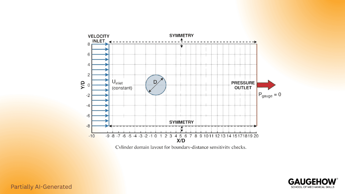
Worked Example 2: Flow over a cylinder with domain sizing and model sensitivity

Bluff-body flow is a clean way to learn what matters because forces are sensitive to domain placement, wake resolution, and whether the physics is steady or inherently unsteady.

Problem setup

Use a 2D cylinder with a diameter D = 0.1 m in air at room conditions. Pick Reynolds number based on intent, because Re ~ 100 behaves very differently from higher-Re turbulent wakes. If you run higher Re with RANS closures, treat force convergence as a primary monitor and consider transient averaging when the wake is unsteady.

Domain extents

Start with upstream 10D, downstream 15D to 20D, and lateral 8D, then test sensitivity by moving boundaries outward.

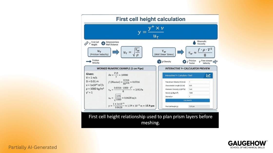
Near-wall first cell height and first-layer sizing

Do not guess the first cell height when wall shear or heat transfer matters. Instead, estimate it from your near-wall target and an estimate of friction velocity, then design prism-layer growth to transition smoothly into the core mesh.

A reproducible estimate for a 1 cm pipe at Re = 10,000

Assume water, D = 0.01 m, Re = 10,000, and V ≈ 1.0 m/s. Estimate the friction factor f ≈ 0.032. Wall shear stress is τw ≈ f ρ V² / 8. Friction velocity is uτ = √(τw/ρ). Kinematic viscosity is ν ≈ 1e−6 m²/s.

Then the first cell height is y = (y+ × ν) / uτ. If you target around 1, y is in microns. If you target around 30, y increases by roughly 30×, which is why wall functions are cheaper.

Embedded y plus calculator (HTML)

Paste your existing y plus calculator embed code here in the web version of the article.

Turbomachinery

You are doing real work, and a review is close. You ran the case, and the plots look clean. But to be honest, clean plots can hide bad physics. Turbomachinery is any machine where a rotor exchanges energy with a flowing fluid, so turbines take energy from the fluid, and compressors add energy to the fluid. (Wikipedia)

What Is Turbomachinery

In plain words, Turbomachinery is the family of rotating flow machines where blades exchange energy with a continuous stream. It includes turbines, compressors, pumps, and fans. (Wikipedia) The unifying idea is not the fluid type. The unifying idea is the rotating blade row doing work on the flow, or taking work from the flow.

This definition matters because it sets the scope. It tells you why the same physics shows up in a Steam turbine and a Centrifugal compressor. It also tells you why wind turbines belong in the same family.

Heat transfer and conjugate heat transfer

When solids and fluids exchange heat and the wall temperature is not known a priori, you may need conjugate heat transfer to solve conduction in the solid and energy in the fluid with matched flux at the interface. The common failure mode is meshing the fluid carefully and treating the solid as an afterthought, which makes thermal resistance and wall temperature mesh-dependent near interfaces.

Transient CFD: when steady assumptions break

Many flows are unsteady by physics, including vortex shedding, rotating machinery, and pulsating inlets. A steady solution can converge numerically and still be wrong physically if the true flow is time-dependent.

A practical approach is to run a steady case for initialization, then switch to transient with a conservative time step, monitor periodic behavior in the decision outputs, and average over several cycles when you compare to experiments.

Tool choices: workflow first

A strong workflow transfers across tools. Differences in meshing, automation, and model availability affect productivity, but defensibility still comes from the same saved artifacts and sensitivity evidence.

Case study: Manifold flow split that looked fine until it did not

Manifolds are a reliable trap because coarse meshes and optimistic near-wall setups can smear separation at splitters. You get smooth contours and nearly equal outlet splits, and then the prototype shows one branch starved.

In reviews, this usually comes down to two corrections: refine the mesh where separation forms, and align the closure model and near-wall treatment with the separation risk. Once you do that, the recirculation region that was previously smeared often becomes obvious, and the predicted split moves toward what the hardware shows.

Naive result versus defensible result

Accuracy and limitations you should state explicitly

This work is strongest when you use it to compare options under the same assumptions, because trend prediction usually stabilizes earlier than absolute prediction. It is also strong when operating conditions are measured, and when the geometry captures the true flow path and the features that drive losses.

It is weaker when the dominant physics is uncertain, for example, with strongly unsteady turbulent separation, poorly known turbulence inputs upstream, multiphase interface behavior, or combustion chemistry. In those cases, you can still use the method, but you should be explicit about what you validated, what you did not validate, and which sensitivities could change the decision.

Templates you can copy into your workflow

Template 1: Run log CSV

run_id,date,cad_version,mesh_cells,prism_layers,first_cell_height_m,y_plus_target,turbulence_model,boundary_conditions,residual_targets,monitors,key_outputs,notes

Template 2: Sensitivity table fields

Conclusion

Computational Fluid Dynamics rewards disciplined setup and honest evidence. If you size the domain to stay out of the physics, plan the near-wall region with intent, and report sensitivity with a clear uncertainty band, you can defend your result even when the problem is complex. The goal is not perfect certainty. The goal is controlled assumptions, bounded numerical error, and saved artifacts that let another engineer reproduce your claim.